Examples¶

Every picture here was drawn by screws itself, from the lines under it. The scripts in examples/ make them all, and each one's guide page says what to look for. The pictures need screws[plot]; in a notebook each animation plays inline, and .save("x.gif") writes it out.

import numpy as np
from screws import robots, se3, so3, viz

# the UR5, and the notes' planar 2R arm with L1 = L2 = 1
ur5, arm = robots.ur5(), robots.planar_2r()

A UR5 sinks a putt¶

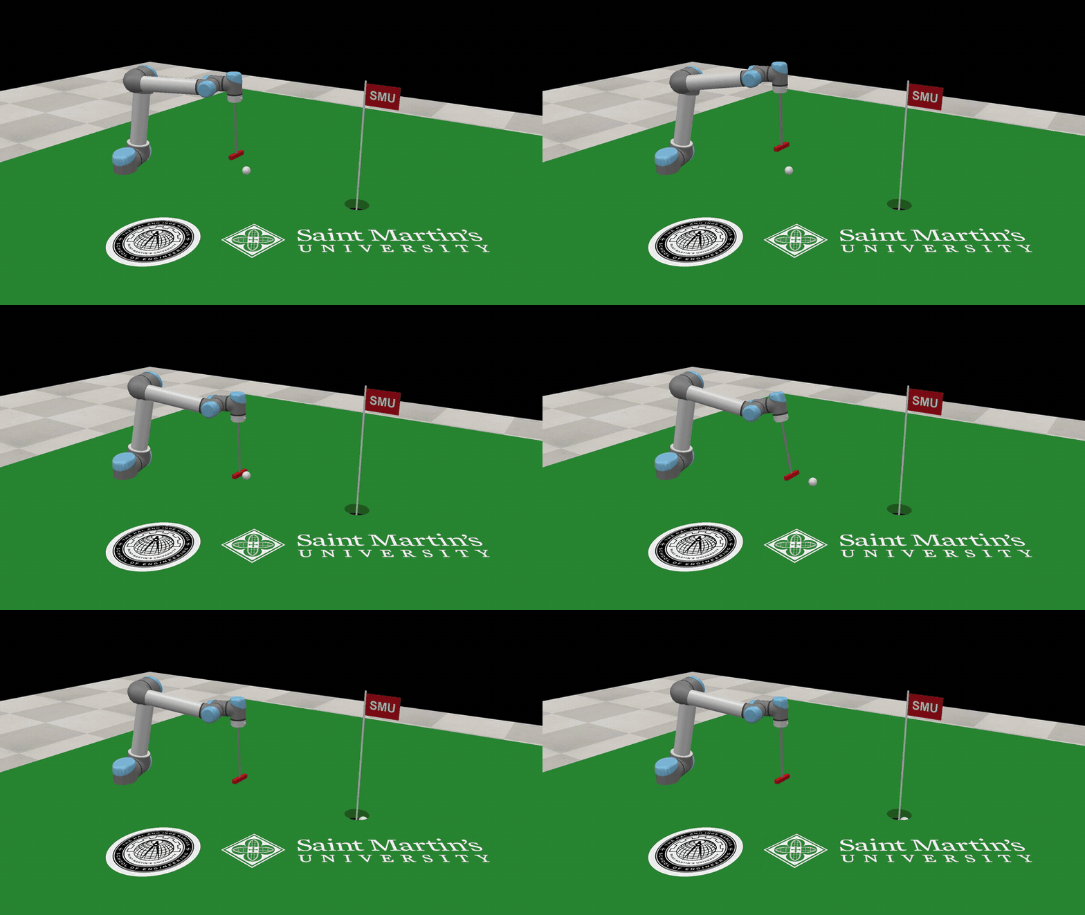
A UR5 in CoppeliaSim addresses a golf ball, swings a putter through it, and the ball drops into the cup

screws.coppelia drives CoppeliaSim. The example builds a green in a running simulator, with a cup cut through the turf, a pin, a ball and a putter on the arm's flange. It then swings the putter through the ball like a pendulum at a chosen speed and reports whether the ball dropped. With --video it records itself.

uv run python examples/putt.py --video putt.mp4

One screw motion from a frame to another¶

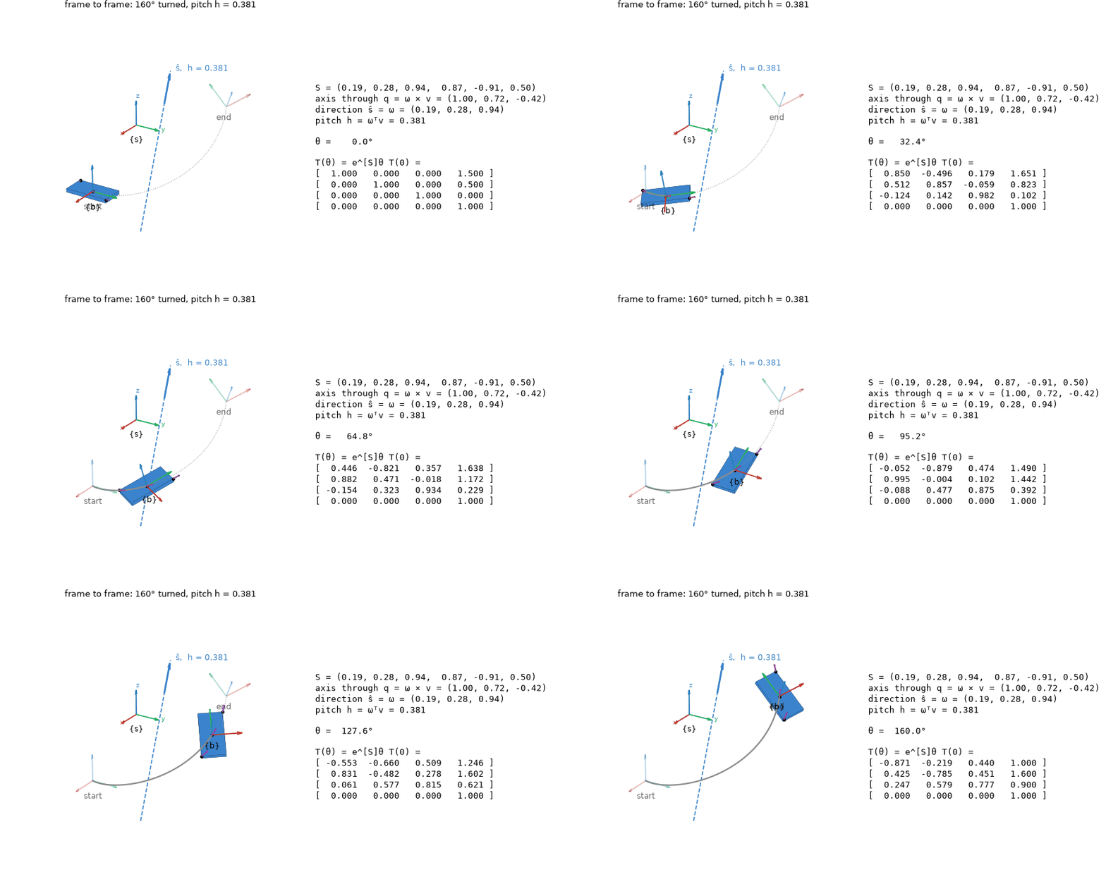
A frame carried to a second frame, with a different origin and orientation, along one screw: its origin traces a helix about the dashed axis

Every rigid-body displacement is a screw motion (Chasles). screw_between finds the one that carries T_start to T_end, and animate_screw plays it, with S, its axis and pitch, and T(θ) beside it.

w = np.array([0.2, 0.3, 1.0]) / np.linalg.norm([0.2, 0.3, 1.0])
T_start = se3.rp_to_transform(np.eye(3), [1.5, 0.5, 0.0])
R_end = so3.exp3(so3.vec_to_so3(np.deg2rad(160) * w))     # 160 degrees about w
T_end = se3.rp_to_transform(R_end, [1.0, 1.6, 0.9])
viz.animate_screw(viz.screw_between(T_start, T_end, name="frame to frame"))

A door, a drawer and a screwdriver¶

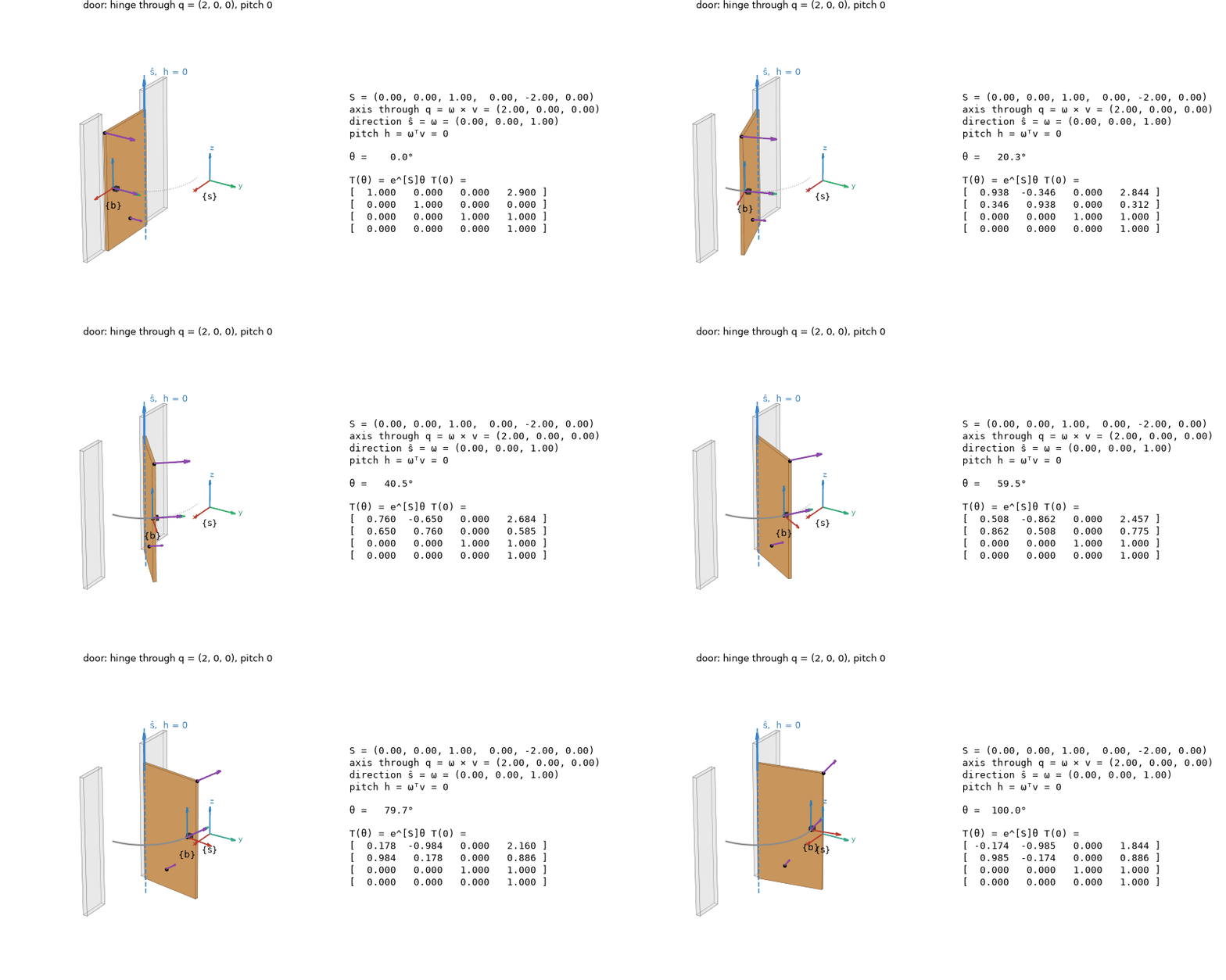
A door swung about its hinge, with its screw axis, the handle's circle and T(θ) beside it

The three pitches: zero (a hinge), infinite (a slide) and finite (a helix).

viz.animate_screw(viz.door())
viz.animate_screw(viz.drawer())
viz.animate_screw(viz.screwdriver())

The space twist and the body twist of one motion¶

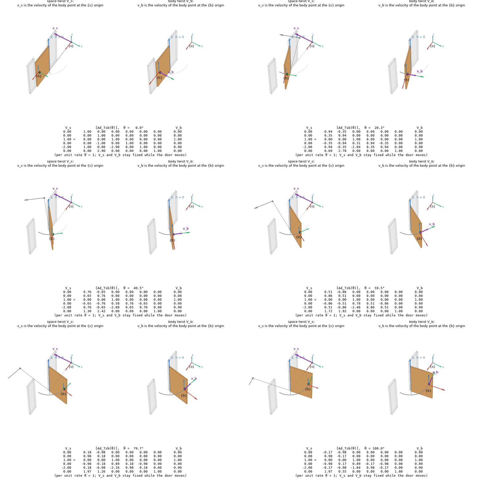
$The door's motion drawn twice: on the left v_s at the origin of {s}, on the right v_b at the handle, with V_s = [Ad_Tsb] V_b underneath$

On the left is V_s, on the right V_b, and underneath them V_s = [Ad_Tsb(θ)] V_b, with the adjoint changing as V_s stays fixed.

viz.compare_frames(viz.door())

Where a joint's screw axis is now¶

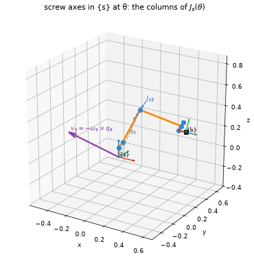
The UR5 at θ with joint 3's current screw axis J_s3 dashed in blue, and v_3 built from the joint's position q_3

axes="current" draws each axis where the joints inboard of it have carried it, which is column i of J_s(θ). "construction" builds that column, J_si = (ω_i, −ω_i × q_i).

theta = [0.3, -1.1, 1.4, 0.2, 0.9, -0.5]
build = ("skeleton", "frames", "axes", "omega", "construction")
viz.draw_robot(ur5, theta, axes="current", joints=[2], show=build)

The Jacobian's columns¶

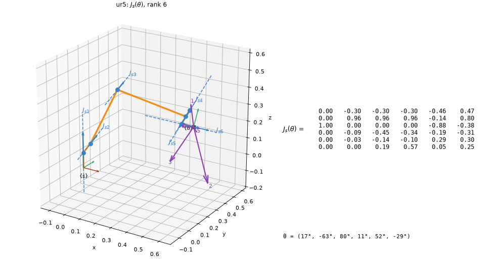
The UR5 with each joint's current screw axis dashed in blue, the tool velocities they give as numbered purple arrows, and J_s(θ) beside it

The dashed lines are the six columns of J_s(θ). The numbered arrows show the velocity each joint alone gives the tool point.

viz.draw_jacobian(ur5, theta)

More in Jacobians and ellipsoids.

An ellipsoid that follows the arm¶

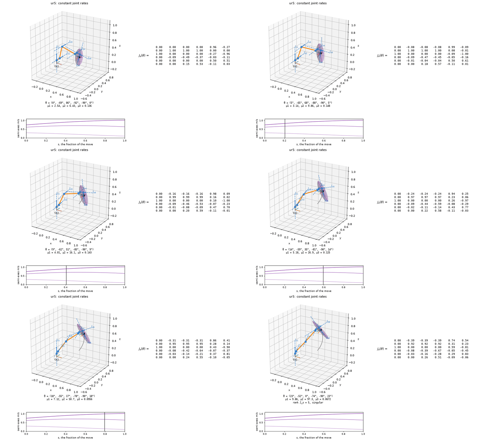
The UR5 straightens its elbow at constant joint rates while its purple manipulability ellipsoid changes and J_s(θ) updates beside it

animate_robot moves the robot at constant joint rates. The axes, the manipulability ellipsoid and the matrix follow it, and the chart underneath tracks the semi-axes. Here the elbow straightens into a singularity, and J_s loses rank.

theta0 = [0, -1.2, 1.5, -1.6, -1.57, 0]
viz.animate_robot(ur5, theta0, [0.4, -0.9, 0, -1.3, -1.57, 0.4], matrix=True)

More in Jacobians and ellipsoids.

Into a singularity¶

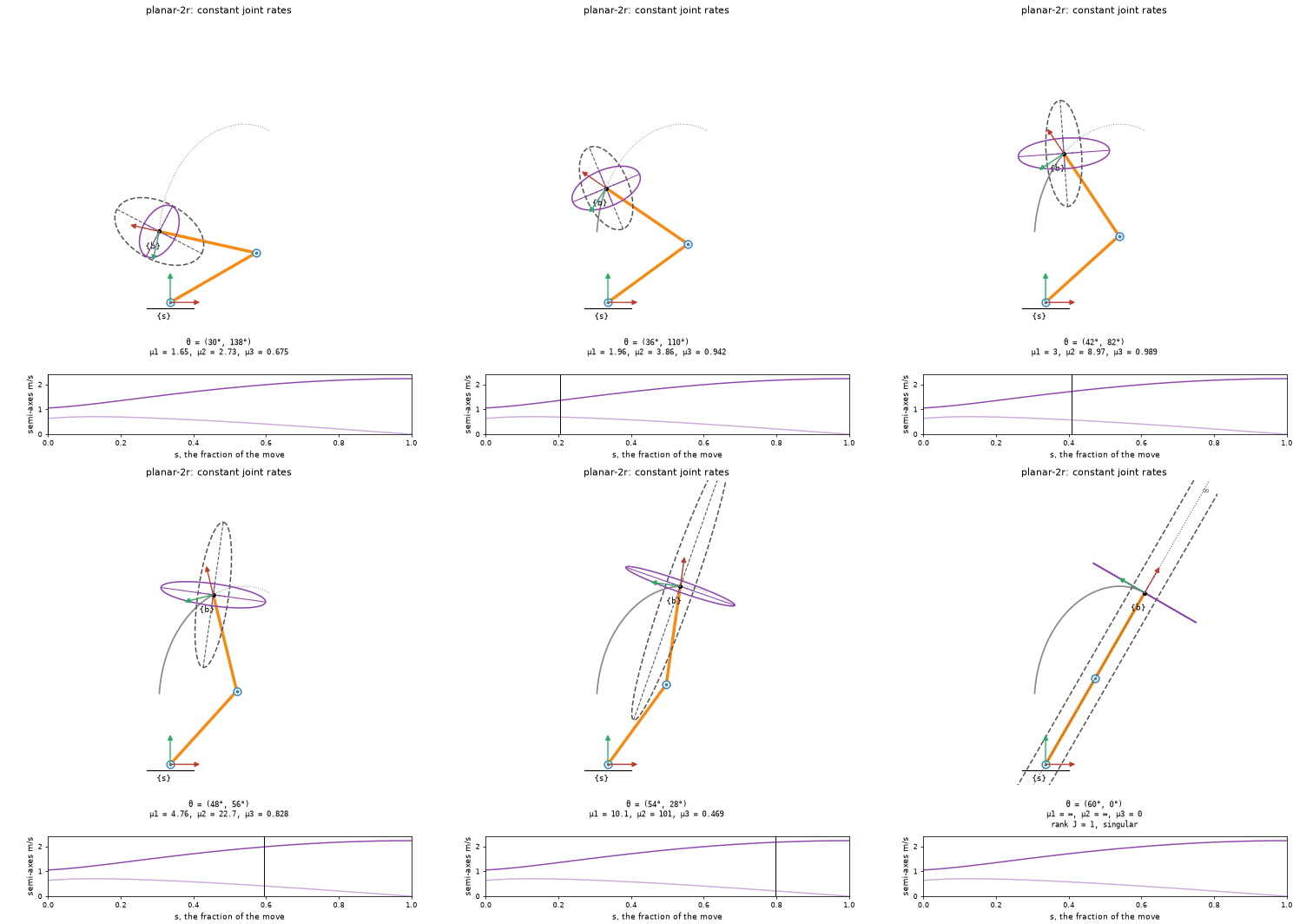
The 2R arm straightens while its purple ellipse thins to a segment; a chart below shows the short semi-axis falling to zero

The 2R arm stretches out straight, and its velocity ellipse thins to a segment.

start, end = [np.pi / 6, 2.4], [np.pi / 3, 0]   # theta2 = 0 is stretched out
viz.animate_robot(arm, start, end, force=True, planar=True)

More in Jacobians and ellipsoids.

Constant joint rates, or a constant twist¶

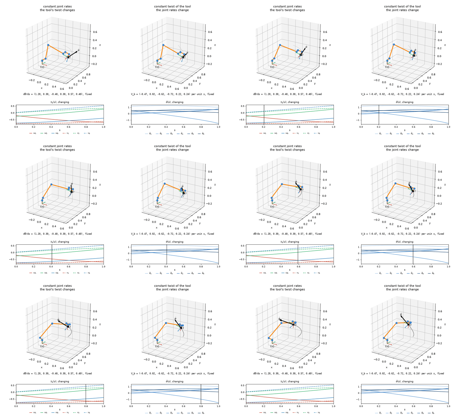
Two UR5 panels from the same start to the same end. Left, constant joint rates with the body twist changing; right, a constant twist of the tool with the joint rates changing

Both panels start and end in the same place. On the left the joint rates are constant and the tool's twist changes. On the right the tool follows one screw motion, and inverse kinematics finds the changing joint rates.

viz.compare_paths(ur5, theta0, [1.2, -0.9, 1.1, -1.3, -1.0, 0.4])

More in Jacobians and ellipsoids.

The same computations as formulas¶

screws.symbolic does the computations in SymPy, so the forward kinematics and the Jacobians come out in the joint variables:

import sympy as sp
import screws.symbolic as sym

L1, L2 = sp.symbols("L1 L2", positive=True)
arm_sym = sym.SymbolicRobot.from_screw_axes(
    sym.trans([L1 + L2, 0, 0]),
    [sym.revolute_axis([0, 0, 0], [0, 0, 1]),    # joint 1 at the origin
     sym.revolute_axis([L1, 0, 0], [0, 0, 1])],  # joint 2 at (L1, 0, 0)
)
arm_sym.fk()[:3, 3]

Matrix([
[L1*cos(theta1) + L2*cos(theta1 + theta2)],
[L1*sin(theta1) + L2*sin(theta1 + theta2)],
[                                       0]])

arm_sym.jacobian_body()

Matrix([
[                  0,  0],
[                  0,  0],
[                  1,  1],
[     L1*sin(theta2),  0],
[L1*cos(theta2) + L2, L2],
[                  0,  0]])

More in Formulas. To compare your own implementation of a function with the library's, see Check your own code; for joint sliders that redraw any of these pictures in a notebook, see viz.explore in Jacobians and ellipsoids.